Time intelligence functions support calculations to compare and aggregate data over time periods, supporting days, months, quarters, and years. In order to use any time intelligence calculation, you need a well-formed date table. All dates need to be present for the years required. There needs to be a column with a Date/Time or Date data type containing unique values. Standard data sources only record dates where an event happened. However, a custom date table provides a continuous timeline, ensuring charts display gaps or zero-value periods correctly instead of skipping them. Thus, the common mistake of reports displaying wrong values due to missing data tables can be avoided.
Upload the data
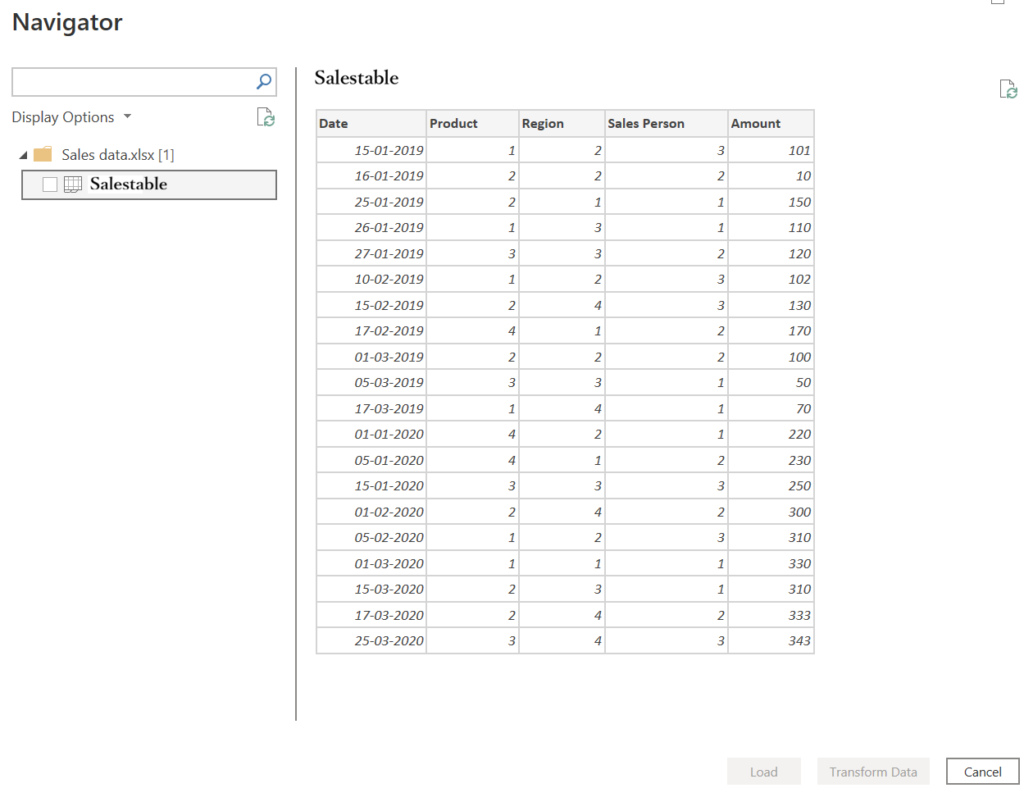
To start with, the Excel data to be analysed can be uploaded using the option Home > Get Data> Excel Workbook. In the data below, you can find non-continuous data being present for the quarter from Jan-Mar in 2019 & 2020, with no data in the subsequent quarters.
Format the data
In the Report view, select the Table visual under Visualizations. Under Data, once the Date & Amount is selected the uploaded excel data will be visible as a table as shown below.
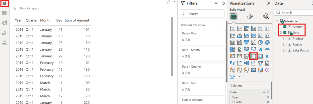
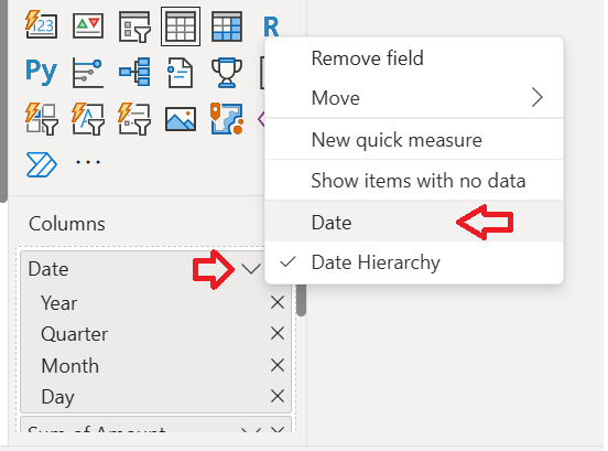
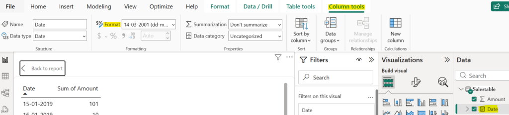
In the above table display, the date is displayed as a hierarchy. This can be corrected by selecting the “Date” option as shown above. Also, the necessary date format can be selected by navigating to the Column tools > Format and choosing from the drop-down as shown below.
Add measures
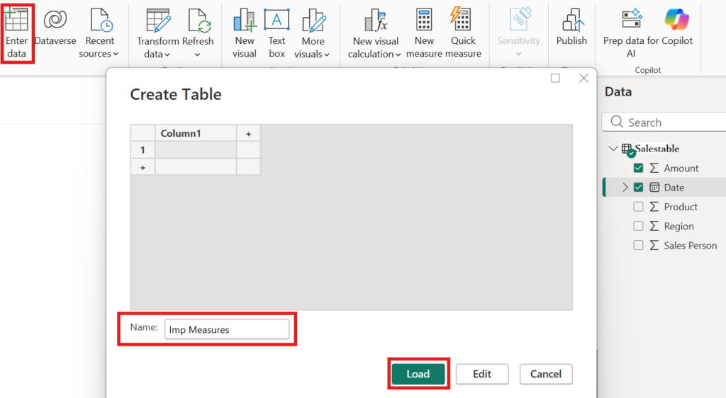
Now that the data is ready, we will move on to adding measures for further calculations. For this, we will start with creating a measures table first. The table can be created by clicking on “Enter data” option under Home tab. Input the name in the field as shown below and click on Load button and your measures table is ready.
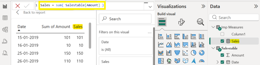
The measures table “Imp Measures” will appear on the right under Data. The first measure,i.e, Sales is calculated by using the DAX formula as highlighted in the yellow frame as shown below. As you can see, the Sales column data is same as the Amount column data. Since both the column data are the same, we will use the Sales measure going forward and hide the Amount column.
The next three measures will be calculated using the below formulas.
Sales YTD = CALCULATE( [Sales], DATESYTD( Salestable[Date] ))
Sales PY = CALCULATE([Sales], DATEADD(Salestable[Date],-1, YEAR))
Sales PY YTD = CALCULATE([Sales PY],DATESYTD(Salestable[Date]))
Here the [Sales] data will be filtered based on the date and displayed in separate columns as Sales YTD, Sales PY, Sales PY YTD using the CALCULATE DAX functions. The point to note here is that we are using the existing date column in our calculations. We will analyse the results in the final section.
Custom Date Table
To create a custom date table, navigate to Home > Get data > Blank query. Using the highlighted Power Query M function List.Dates, create the custom date table for the years 2019 & 2020. In the M function, the start date(2019,1,1), number of days(2 years -> 730days) and the duration(1 day interval between the dates) parameters are specified.
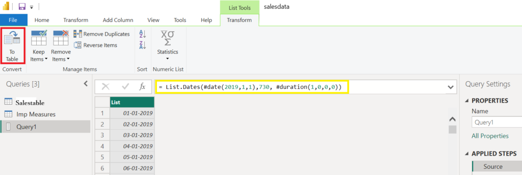
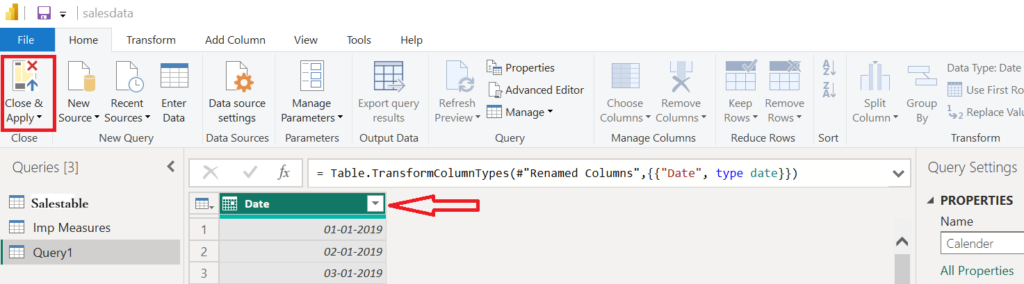
Rename the column name to Date from List and click on the Close & Apply button at the top left.
Connecting the Tables
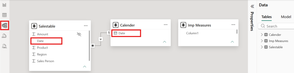
Now that we are ready with the custom date table, we can connect it to the Salestable date as shown in the figure below using the one-to-many relationship.
Add new measures using the Custom Date Table
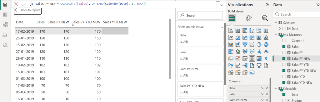
Now that the connection is made between Salestable and the new Calendar, we will calculate the following same three measures but with new calender table created earlier.
Sales YTD NEW = CALCULATE( [Sales], DATESYTD( Calender[Date]))
Sales PY NEW = CALCULATE([Sales], DATEADD(Calender[Date],-1, YEAR))
Sales PY YTD NEW = CALCULATE([Sales PY NEW],DATESYTD(Calender[Date]))
The point to note here is that we are using the new date table in our calculations ,i.e, to calculate Sales PY NEW, Sales PY YTD NEW and Sales YTD NEW.
Compare the Results
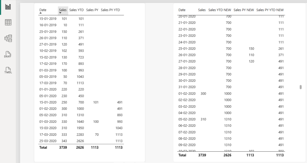
In the below figure on the left, we have the table of data generated using the existing date column. As you can see, there is no data in the Sales PY & Sales PY YTD columns for the year 2019 and a few rows are populated in the Sales PY column for the year 2020. However, as there is Sales data present in each of the rows in 2019, we should have seen data in many rows for Sales PY in 2020. For example, on 01-02-2020, we see no data under Sales PY. If we check the previous year(PY) data on the same date, we are unable to find any corresponding data. Hence, the data section is blank for these dates under Sales PY, which is not appropriate.
If you compare with the table on the right(created using the calendar table), the Sales YTD for 15-01-2019 & 16-01-2019 is 101 & 111 respectively in both the tables. However, as there was no sales between 17 – 24th, there is no dates/data displayed in the table on the left, but on the right as the dates are continuous, the Sales YTD data of 111 continues till 24th.
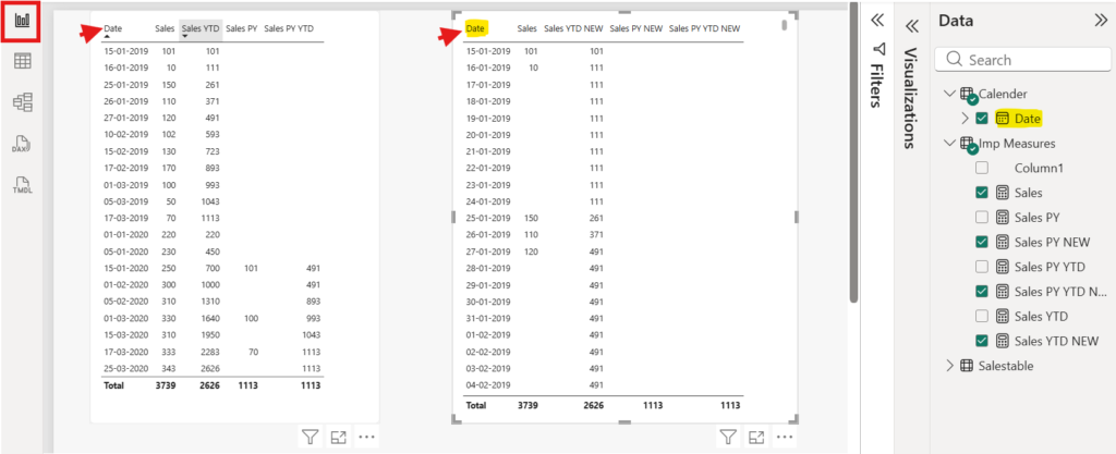
In the below figure on the right, you can see the data distribution for Sales YTD NEW, Sales PY NEW, Sales PY YTD NEW in the second half of 2020, generated using the newly created date table.
Plot a Graph
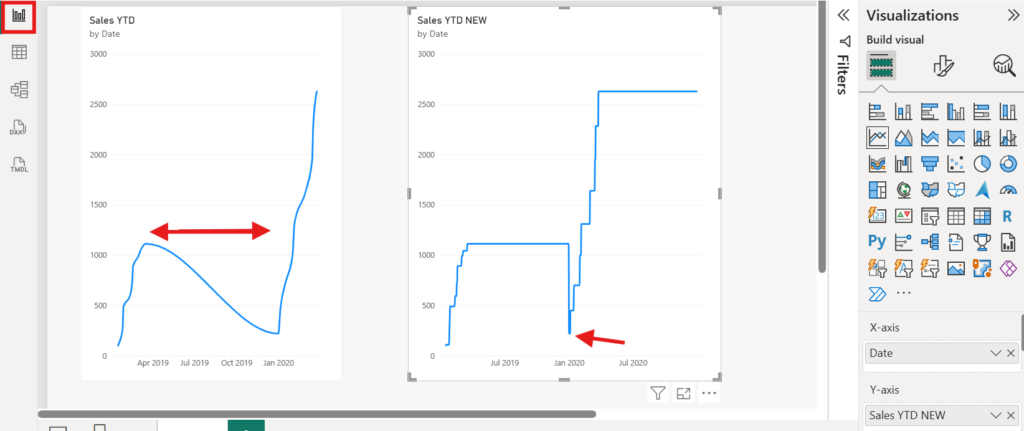
To better understand the concept, let us make use of the line chart visual. The parameters being date & Sales YTD (left graph), date & Sales YTD NEW (right graph). The left-side graph depicts the line moving towards zero as there was no sales between April to December 2019. However, the right-hand side graph was plotted for the data generated from the Calendar table. You can see that the line is steady between April to December 2019 during which there was no sales, hence the depiction is proper. At the end of the year, 2019 you can see the line drop to zero and rise again in the new year, 2020.
Further Reading:


Leave a Reply