Predictive analytics helps us understand potential future occurrences by analysing historical data. Machine learning (ML), on the other hand, is a subset of artificial intelligence (AI) that enables machines to learn from large datasets and identify patterns without being explicitly programmed for every task. A common misconception is that predictive analytics and machine learning are the same, but they are distinct concepts. The area where these two disciplines intersect is known as predictive modelling.
Machine Learning Types & Workflow
As a subset of AI, machine learning in its most elemental form uses algorithms to parse data, learn from it, and then make predictions or determinations based on the use case. Different algorithms are needed for different problems and tasks, and solving them depends as well on the quality of the input data and power of the computing resources.
There are three types of Machine Learning
- Supervised Learning: The model is trained on labeled data (input and correct output provided). Common algorithms include Linear Regression and Decision Trees.
- Unsupervised Learning: The system finds hidden patterns in unlabeled data, such as clustering customers into segments based on behavior.
- Reinforcement Learning: An agent learns by interacting with an environment, receiving rewards or penalties to determine the best strategy (e.g., AlphaGo).
Ideally, a Machine Learning project follows a six-step workflow as follows.
- Data Collection: Gathering relevant raw data.
- Feature Engineering: The most critical stage involves data cleaning and pre-processing to prevent “hallucination”.
- Model Selection: Choosing an algorithm suited to the specific problem.
- Model Training: Typically splitting data into 80% for training and 20% for testing.
- Model Evaluation: Measuring accuracy using metrics like F1 score or R-squared.
- Model Deployment: Integrating the model into a real-world production environment.
Supervised Learning
Here our focus will be on Supervised Learning. Supervised learning is defined as a technique where a model is trained on a labeled dataset containing the “correct answers” or ground truth. It is compared to a teacher-student relationship, where the model learns the underlying logic from provided examples to solve new, unseen problems.
Primary Branches
Supervised learning is categorized based on the nature of the target output:
- Regression: Used for predicting continuous values or quantities, such as price, age, or temperature. It aims to establish a mathematical relationship between independent variables (features) and a dependent variable (target). Line of regression shows the relationship between the 2 variables.
- Classification: Used for assigning observations into predefined categories or groups, such as “Spam” vs. “Not Spam” or “Yes” vs. “No”. It works by identifying a Decision Boundary to separate different classes.
Key Algorithms
The sources list several algorithms tailored to different data complexities:
Regression Algorithms
These include the following
- Linear Regression (straight-line relationships)
- Polynomial Regression (extn of Linear regression, data not linear but follows a curved patterns)
- Ridge and Lasso Regression (used to prevent overfitting)
- Support Vector Machines (SVM/SVR) (effective for non-linear data)
Classification Algorithms
These include Logistic Regression (predicts probabilities for binary classification), Decision Trees (uses condition-based splits – used for classification & regression), Random Forest (combines multiple trees), K-Nearest Neighbor (KNN) (a “lazy learner” based on proximity), and Neural Networks (modelled after the human brain for complex tasks like image recognition – used in Deep Learning).
Overfitting & Model selection
Overfitting occurs when a model learns the “noise” or random fluctuations of the training data instead of the actual concept, leading to poor performance on new data. The sources offer actionable strategies for choosing the right model based on the dataset:
- Simple/Linear Data: Use Linear or Logistic Regression
- Need for Interpretability & Visual representation: Use Decision Trees
- For overfitting & large datasets: Use Random Forest
- Large/Complex Data: Use Neural Networks
- Small/Simple Datasets: Use KNN
Evaluation Metrics
To measure model performance, the sources outline specific metrics:
- Regression Metrics: Mean Absolute Error (MAE), Mean Squared Error (MSE), Root Mean Squared Error (RMSE), R-Squared (R²) etc. There is no single best metric for evaluating the performance of a regression model. The metric chosen for a use case will depend on the data used to train the model, the business case you are trying to help, and so on.
- Classification Metrics: Accuracy, Precision, Recall, F1 Score, etc. The choice of a metric(s) depends on the problem at hand, the cost of false positives and false negatives, and the level of imbalance in the dataset.
Predictive analytics and machine learning go hand in hand, as predictive models typically incorporate a machine learning algorithm. These models can be trained over time to respond to new data or values, delivering the results the business needs.
LinearRegression Predictive Model
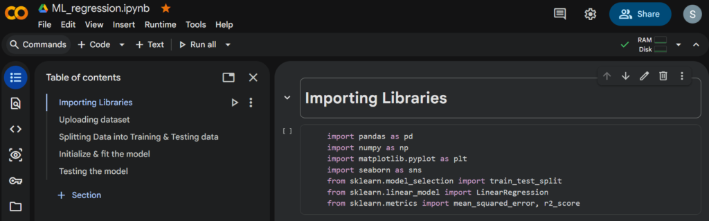
Here, we will be using the Python development environment is Google Colab, a cloud-based platform that requires no local installation. Code runs on remote server in Google’s data centers. Unlike standard .py files, notebooks(.ipynb) allow for a combination of executable code cells and formatted text cells.
The first part of the code will include the section to import the libraries. The SciKitLearn library, which we use in the code, is geared towards machine learning. Here, we will just be doing linear fits; however, Scikit-learn has many different models built in. Since we will be looking into linear regression, we will import the LinearRegression model from SciKitLearn library. This type of model performs ordinary least squares fitting. You will first import the model, then you will create a model object. After creation, you will give data to the model and tell it to perform a fit. Your model can then be used to make predictions. The same is depicted in the following code.
You can find the full code link here and the data to train and test the model as follows.
As you can see in the Table of contents picture above, the first step is importing the libraries followed by uploading the dataset. The dataset should then be checked for missing values, and any missing entries should be removed to ensure data quality. Converting text to numerical format and ensuring column order is correct are vital for avoiding “glitches” or model failure. The data will later be split into training and testing data using the python code. In the next steps, we will create the linear regression model and train/fit the model with the data. Once done, we will test the model based on the output Mean Squared Error and R-squared values. Finally, we will provide our data to check the predicted values.
It is important to note that the most complex algorithm is not always the best choice. When the same dataset was evaluated using the Random Forest model, it produced significantly poorer performance, with Mean Squared Error (MSE) and R-squared values compared to the linear regression model.
Machine learning can predict prices accurately if given sufficient historical values. Models like this can be deployed for public use using tools like Streamlit. Refer to the link below to learn more about Streamit.
Get started with Streamlit – Streamlit Docs
References:


Leave a Reply