In case you are familiar with MS Excel, by first look you might feel that Google Sheets and Excel are similar. Though it is true to some extent, however you need to know a few things in order to utilize the free online application to its fullest. People familiar with Excel might find it easier to work with but one needs to know the appropriate option to select for a certain operation that may be different from Excel. In this blog i have tried to highlight some of the frequently used Excel operations and the way to realize the same in Google Sheets. In order to work with Google sheets, first thing is to be ready with the tool, i.e, we need to logon to Google Drive using the following link; https://drive.google.com/drive/my-drive
Once we login we have the My Drive home screen wherein we can find two subsections namely Quick Access & Name. In the Name subsection we have the list of all files or folders in Google Drive. Next we will be dealing with creating a new spreadsheet and uploading an existing sheet.
Creating / Uploading a Spreadsheet
- In order to create a new spreadsheet we need to right click on the area next to Name subsection, we will get options like Google Docs, Google Sheets, Google Slide among others. As we move to Google Sheets>Blank spreadsheet/From a template, clicking on “Blank spreadsheet” will open an “Untitled spreadsheet” in a new tab. We can specify any desired name by clicking on the “Untitled spreadsheet” area on the top left. Now we are ready to work on the sheet. In case we click on “From a template” we can select from a range of templates like Team roster, Employee shift schedule etc., from the template gallery.
- In order to upload an existing file, first thing is to check the settings of google drive. Click on the setting icon at the top right of the home screen. For the Convert uploads option, tick on the Convert uploaded files to Google Docs editor format. In case this is not checked the uploaded file will be in the original format ,i.e, excel or open office format. Once this is done, click on the “New” button on the top left of the home screen and navigate to “File upload”, select the appropriate file to upload it. We can monitor the upload progress at the bottom right of the screen. One thing to note is that the contents of the uploaded file may undergo some changes due to Google Docs format conversion. So, make sure to check the contents and make appropriate changes once the file is uploaded.
Formatting a sheet
Once we have the sheet on hand, we can start working on it and format using any of the following options available. Lets say we want to format a table, we can use the numbered options 1 – 7 as shown in the below figure – to change the currency to dollars, decimal position/rounding, merging cells, vertical formatting the contents, text wrap, rotate the text, font selection etc., We can assign colors to the table by navigating to Format>Alternating colors wherein we can select from a range of existing table coloring formats. We have the provision to select from a range of currencies available by clicking on the 123>more formats option next to the option 2.
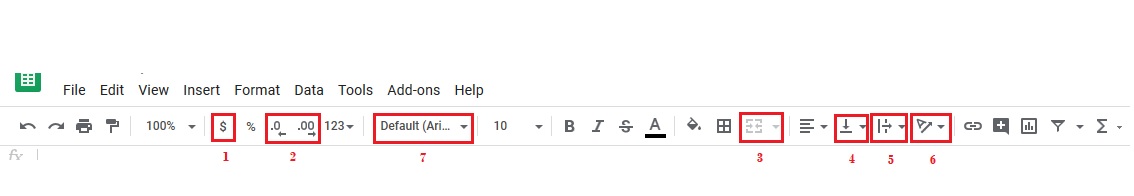
Few Formatting Options
Cell Referencing, Operators and Functions
Incase we are familiar with MS Excel, then the cell referencing part is the same in Google sheets as well except for the linking from another file part. The relative & fixed referencing part is the same as in MS Excel. The linking to another sheet is also the same wherein we use the equation “=’other sheet name’!cell reference”. However, the linking to another file has some changes wherein we use the function IMPORTRANGE(“link to the other file”, “cell ref”). Here we get the link of another google sheet by clicking on the Share button when we open the other file.
Next moving on to the operators and functions part, there is no change in operators as we can use the same ones used in MS Excel. Regarding formulas, we can insert a formula by navigating to Insert>Function>.. or by typing the formula manually in the cell. Some of the frequently used functions are AVERAGE, SUM/SUMIF/SUMIFS, COUNT/COUNTA/COUNTIF, TODAY/NOW, CONCATINATE to name a few.
Sort and Filter
Sorting and Filter can be done by 2 methods in Google sheets, one is through the menu and another method is through formulas or functions. Lets first use the menu method to sort. Select the table to sort and navigate to Data>Sort range. A pop up window opens wherein we can specify the sort by column from the drop down list available. Here multiple columns can be specified as well. Next moving on to the filtering part, select the whole table to be filtered then navigate to Data>Filter. We can see that an inverted triangle icon shows up in each column header. Just click on the inverted triangle to filter the respective column and the whole table by either values and/or condition. The filter can be turned off from the menu by navigating to Data>Turn off filter.
Next method is using functions to sort/filter. The functions being; sort(…..), filter(…..), sortn(…..). Each of these functions create a separate table and can be deleted only from the cell wherein the function was typed in.
Share
Sharing of sheets on google is easy, just click on Share button at the top right corner or navigate to File>Share which will open the following window.
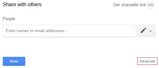
Clicking on Advanced button will open Sharing setting window wherein we can select options like who can access the sheet like public/private, invite the people who can have access to either edit/comment/view the sheet, disable options to download etc.,
Pivot Table
As we are familiar about pivot tables in excel, the same logic works here on a long list of data with no empty spaces in between. Navigating to Data>Pivot table will give us a blank pivot table sheet to work on. The pivot table editor on the right will gives a few choices of simple pivot tables to choose from based on google’s AI prediction. However, those choices are limited and we need to customize the Rows, Columns, Values and Filter section on the right to pull out the desired data. Once the table is generated, if we want to further detail on the rows, for example displaying dates as years – just right click on any date cell and select create pivot date group and choose any appropriate option.
Macros
Another functionality similar to the one found in Excel. If we are to perform the same kind of operation on a spreadsheet again and again, it is best to use a macro to automate the steps and save time. Navigate and click on Tools>Macros>Record Macro. This action opens a pop up at the bottom of the screen showing a flashing red dot, under which there is a provision to select either the absolute/relative referencing. To start recording, just perform the necessary steps on the google spreadsheet. Once done, click on the save button at the bottom pop-up and give an appropriate name.
In order to execute a saved macro on a new non-formatted spreadsheet, just navigate and click on Tool>Macros>”New macro name” to format the spreadsheet right away.
Drop Down Lists & Checkbox
This feature in Google sheets is similar to the one is Excel. Select the range of cells on which the drop down list needs to be inserted. Navigate to and click on Data>Data validation, we get the below pop-up window.
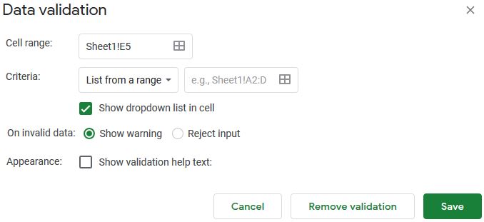
Under Criteria, select List of items and insert the appropriate text separated by comma to be displayed as part of drop down list. Click on Save and we have the list as part of drop down. Under Criteria we have other options like Number, Text, Date, Checkbox etc.,that can be selected based on our needs. In case we need other special characters to be inserted into the drop down we can pick them up from Google Docs>Insert>special characters.
Credits:
Online Materials


Leave a Reply